Why your inverter lies about LFP state-of-charge — and how our software second opinion became the number that runs the house

TL;DR

If you run a home battery on LiFePO₄ (LFP) cells — a Sungrow, Deye, Sunsynk or anything sold as “Solar Battery Storage from China” — your inverter’s state-of-charge reading is probably wrong by 10–15 % after two weeks. Ours managed something better: in a single week it read 100 % while the pack was truly about 96 %, and then 0 % for days while roughly 45 kWh of real charge sat in the cells. One night it spent eight hours firing discharge bursts every five minutes from a battery it believed was empty.

We built a software “second opinion” SOC sensor on the Home Assistant box that already runs the house — a Plett-style Dual Extended Kalman Filter with a current-bias state. The first version of this write-up ended with the estimator in shadow mode and a known weak spot below 30 %. Since then the project pivoted: instead of hand-tuning the filter, we wrapped it in a self-calibration layer that learns the pack’s real capacity, current bias and OCV curve from ordinary daily operation. Its first two-point capacity closure fired on 8 June and measured the pack at 1808.7 Ah usable against a 2100 Ah nameplate. On 10 June we re-pointed the household optimiser (EMHASS) from the inverter’s SOC to ours. The second opinion is now the number that runs the house — with the inverter demoted to a cross-check, and a hardware BMS that remains the only safety floor.

This post is the field write-up: why the BMS gets LFP wrong, what we built, how it taught itself the pack, what it caught, and what guards it.

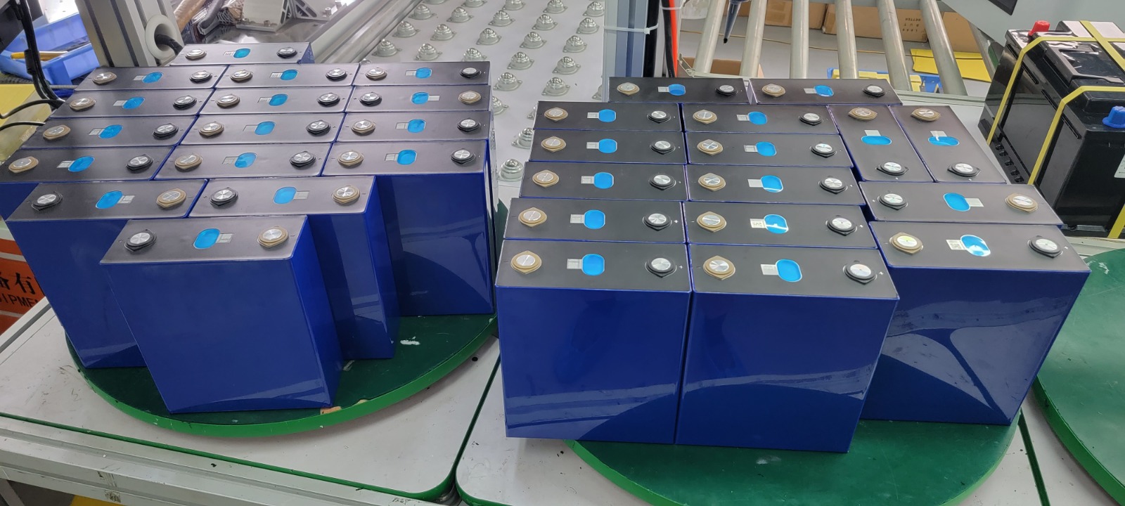
Prismatic LFP cells of the type the system in this post is built on — 16 in series, 21 strings in parallel, ~107.5 kWh nameplate. Same chemistry, same flat-OCV plateau between roughly 20% and 90% SOC, same engineering problem the DEKF estimator is built to address.

The LFP plateau problem in one paragraph

Lithium iron phosphate cells have a near-flat open-circuit-voltage curve from roughly 20 % to 90 % state-of-charge. Across that whole band the per-cell voltage sits at about 3.30 V and barely moves — dOCV/dSOC is close to zero. Voltage is useless as a SOC indicator in the plateau. The only places voltage carries usable information are the steep “knees” below ~20 % and above ~90 %.

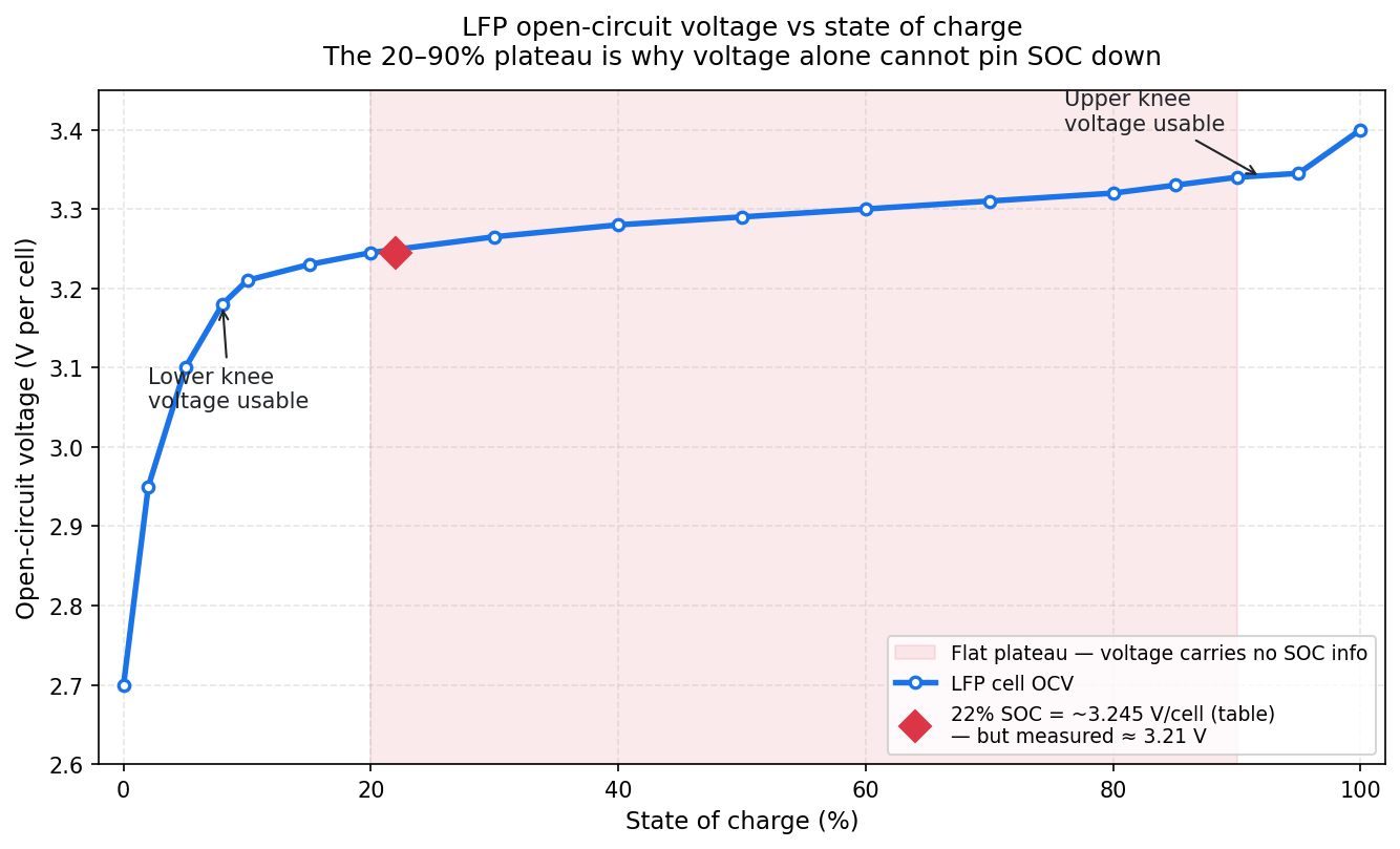
Per-cell OCV plotted from the table in the deployed estimator. The shaded band — 20% to 90% — is where the cell sits 90% of the time, and where voltage tells you almost nothing about state of charge.

That leaves coulomb counting: integrating measured current over time. The inverter’s internal current shunt has a typical bias of ±0.5–1 %. Bias integrates monotonically and never self-corrects. Across two weeks of normal cycling it compounds to the 10–15 % drift we observe — and the error gets violently worse whenever the counter is re-anchored from a bad reference. ACCURE’s field study across 12 GWh of operating battery storage found exactly this picture industry-wide: ±15 % typical BMS SOC error on LFP, with outliers above 40 %.

The textbook fix is to “snap” SOC to the OCV table whenever the pack is genuinely at rest and not in the plateau — same trick BYD uses in EVs. That requires being able to recalibrate from outside the BMS. The Deye exposes no such hook.

Why this isn’t an academic problem

On 2026-05-18 our cells reached 47.7 V at the pack (≈ 2.98 V/cell) before the hardware BMS over-discharge floor cut in. The cause was straightforward: the inverter’s SOC reading said the pack still had useful energy. The home-energy optimiser believed it and scheduled further discharge against high evening Amber prices. The cells were already in the lower knee. No permanent damage — the hardware floor did its job — but a software estimator should never be the layer keeping cells away from the BMS limit.

The principle this near-miss surfaces, and which governs everything that follows: software never relaxes a hardware limit. The hardware BMS is the non-negotiable safety floor; software only optimises within the envelope the hardware enforces. Any “improved SOC sensor” that sits between the inverter and the optimiser is an optimisation correctness device, not a safety device. The hardware floor stays the hardware floor.

And three weeks after that near-miss, the inverter produced the clearest possible demonstration of why the project exists.

The week the inverter read 100 % and 0 % — for the same pack

The chart below is one week of live telemetry, ending the morning this revision was written. The purple trace is our estimator; the orange trace is the Deye’s own SOC register.

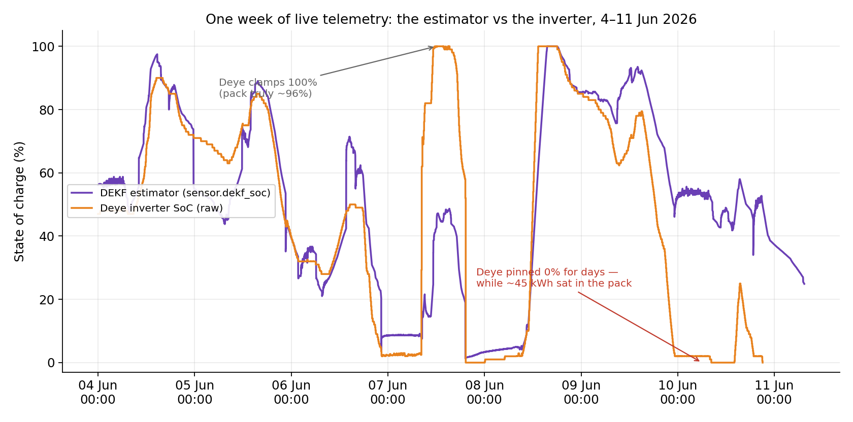
Seven days, two SOC readings of the same physical battery. Early in the week the inverter clamps 100 % while the pack is truly around 96 %. From the 9th it pins 0 % — for days — while the estimator correctly tracks ~45–55 % and the house keeps drawing real energy from the “empty” battery. Both failures are the same coulomb-counter pathology, in opposite directions.

This is not a subtle disagreement that needs statistics to see. The inverter’s counter had been mis-anchored after a settings change and walked a 50-point error in three days. Any optimiser planning against the orange line is planning a fiction: it will burn grid import protecting a battery that is half full, and it will happily discharge a battery that is nearly empty — which is exactly the 18 May near-miss.

The night the “empty” battery fired 64 discharge bursts

The mis-anchored counter didn’t just produce a wrong dashboard number. Overnight on 9–10 June it produced eight hours of synchronized hardware oscillation.

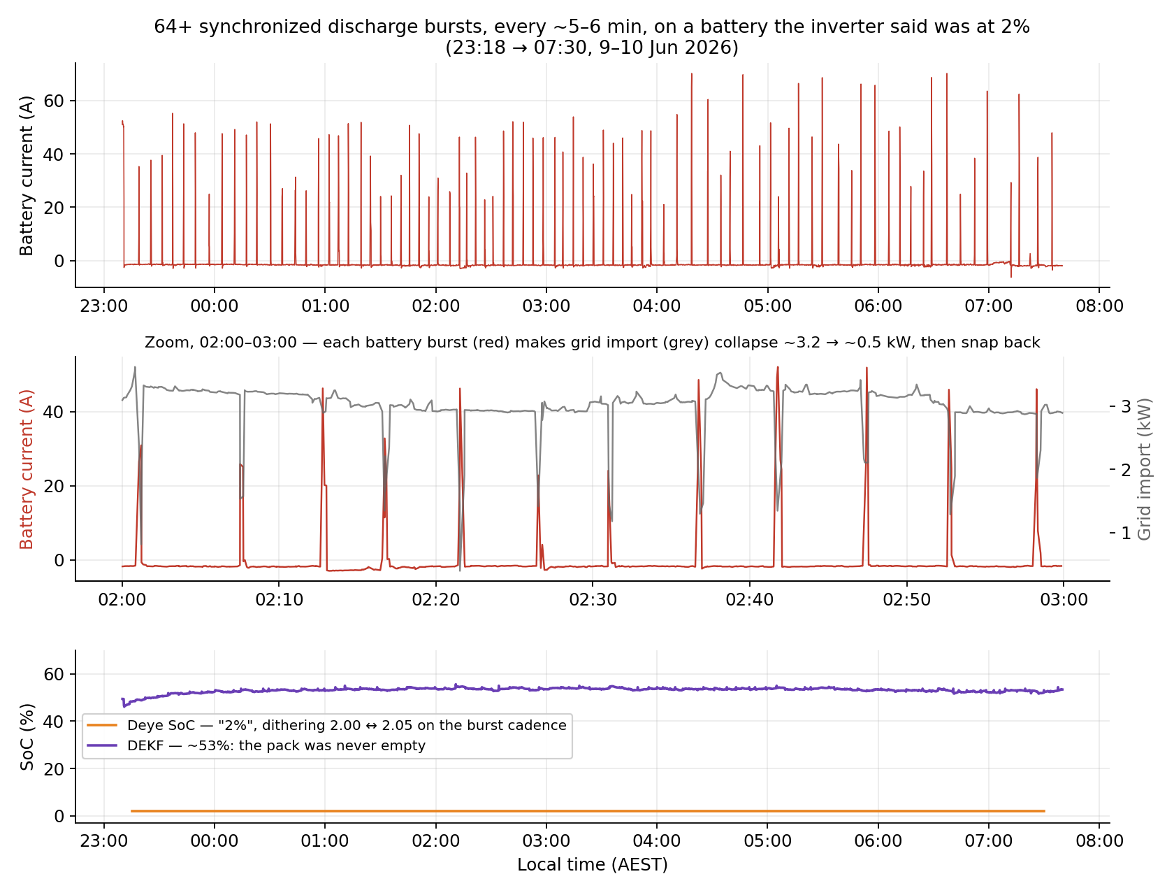
The 5-minute limit cycle, from the recorder. Top: the full night of discharge bursts. Middle: a one-hour zoom — each battery burst (red) makes grid import (grey) collapse and snap back as the inverters flip between “battery empty, import everything” and “battery has charge, carry the house”. Bottom: why — the Deye believed 2 % while the estimator (correctly) read ~53 %.

The mechanism is a classic control failure: the Deye’s time-of-use SOC floor has no hysteresis — the same threshold enables and disables discharge. The mis-anchored counter sat exactly on the 2 % floor, a small float charge crept it to 2.05, discharge re-enabled, the house load stepped on, the counter dropped to 2.00, discharge cut off, and the cycle repeated every five to six minutes from 23:18 to 07:30. Two inverters on a shared pack flapped in perfect sync. Meanwhile the house imported ~3 kW from the grid all night — paying for energy that was already sitting in the battery.

Two lessons worth stealing even if you build none of what follows: a threshold with no hysteresis plus a value resting on it is a guaranteed limit cycle, and a coulomb counter is only as good as its last anchor.

What we built

A second SOC sensor — sensor.dekf_soc — running as an AppDaemon app on the same Home Assistant Green box that already runs all our automation, publishing a fresh value every 10 seconds. Inside is a Plett-style Extended Kalman Filter with three state variables:

x = [ SOC, V_RC, b_I ]

• SOC — state of charge (0–1)
• V_RC — voltage across the single RC polarisation branch
• b_I — current-measurement bias (the “Dual” in Dual-EKF)

The measurement model is the standard equivalent-circuit form:

V_terminal = N_cells × OCV(SOC) − (I − b_I) × R0 − V_RC

Three details made it actually work where the textbook version stumbles on LFP.

The first is current-gated measurement noise. Under heavy current the dominant error is the IR + polarisation model, not voltage-sensor noise — so we inflate the measurement noise covariance R_MEAS with current. At rest the voltage update is fully active; under heavy discharge or charge it is effectively switched off, leaving coulomb counting to dominate:

# Current-gated measurement noise: trust voltage when at rest,
# distrust it under heavy current where ECM model error dominates.
ai = abs(i_meas)
if ai <= self.GATE_I_LOW:          # |I| <= 2 A
    r_meas_eff = self.R_MEAS       # (20 mV)^2 = 4e-4
elif ai >= self.GATE_I_HIGH:       # |I| >= 10 A
    r_meas_eff = self.R_MEAS_HIGH  # 1000 V^2 — voltage update effectively off
else:
    t = (ai - self.GATE_I_LOW) / (self.GATE_I_HIGH - self.GATE_I_LOW)
    r_meas_eff = float(np.exp(np.log(self.R_MEAS) * (1 - t)
                              + np.log(self.R_MEAS_HIGH) * t))

The result: roughly 86–90 % of the time the filter runs gated — coulomb-counting only — which means the calibration of pack capacity is critical. That observation reshaped the whole project; we come back to it in a moment.

The second is the rest-voltage anchor. The only reliable absolute SOC reference on LFP is a properly rested pack. We watch for sustained low current and snap SOC from an inverse OCV lookup when it happens — but, after one painful lesson, only in the steep zones. A rest-anchor taken in the flat plateau injects the OCV table’s own millivolt-level errors as a ±10 % SOC jump. The current rule: anchor only below ~18 % or above ~88 %, or where the local OCV slope is steep enough to carry real information.

The third is capacity calibration. Coulomb counting divides integrated Amps by pack capacity — so the assumed capacity has to be right or the integration silently drifts. Nameplate said 2100 Ah (16s21p × 100 Ah cells). Early anchor-to-anchor integration said ~1750 Ah. The self-calibration layer below now maintains this number continuously, and its first proper closure measured 1808.7 Ah — ≈ 92.6 kWh effective vs 107.5 kWh nameplate, a ~14 % shortfall, with parallel-string mismatch the leading hypothesis rather than dead cells.

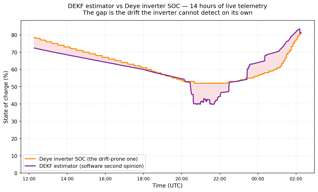
Where it started: the original 14-hour shadow-mode comparison (21–22 May, 3,293 points). The Deye bottoms out around 52 %; the DEKF reads 39.6 %. The shaded gap is drift the inverter cannot detect from coulomb counting alone. Compare with the one-week chart above — by June the same gap had grown from ~12 points to 50.

The pivot: stop tuning the filter, teach it to calibrate itself

The first version of this post ended honestly: the estimator was trustworthy from ~40 % to 100 %, excellent near full, and had a documented failure mode below 30 % — after a deep discharge it could drag a correct ~22 % reading down to ~9.7 % and hold it low for hours. An external technical reviewer (Grok, in critic mode) called the v1 design “~80–90 % of the way to production-grade” and we planned a list of filter upgrades.

Working through that list surfaced the real diagnosis, and it changed the strategy. The Kalman machinery was healthy; the parameters were stale. The hardcoded series resistance (2.5 mΩ) was nearly a third of the pack’s true effective resistance, the OCV table was a generic LFP curve rather than this pack’s, and the capacity was a hand-estimate. A filter with wrong constants doesn’t need a cleverer filter — it needs a mechanism that keeps the constants true. So instead of hand-tuning, the project pivoted to a self-calibration layer: a second AppDaemon app that watches the same telemetry and continuously learns the pack.

It does four things, all from ordinary daily operation:

• Harvests rest points opportunistically. Whenever the pack genuinely rests in a steep zone, it records a clean OCV point and nudges only the steep knots of the OCV table — the plateau stays frozen, because plateau “information” is noise.
• Closes the capacity loop with two-point coulomb closures. Catch the pack rested at a known low point, catch it again rested at a known high point, and the Amp-hours integrated between them measure capacity and current bias jointly. The first closure fired on 8 June: capacity 1750 → 1808.7 Ah, current bias 0 → −1.5 A. That bias number matters: an uncorrected error of that size integrates to a couple of percent of SOC per day — the two-week 10–15 % drift, explained from first principles.
• Tracks resistance online with a recursive least-squares estimator, so the IR correction follows temperature and ageing instead of a constant from a spec sheet.
• Grades its own homework. A 0–100 % confidence score, published as a sensor, that rises with fresh anchors and clean closures and decays as calibration goes stale. It sits in the 70s in normal operation and peaks near 100 just after a closure.

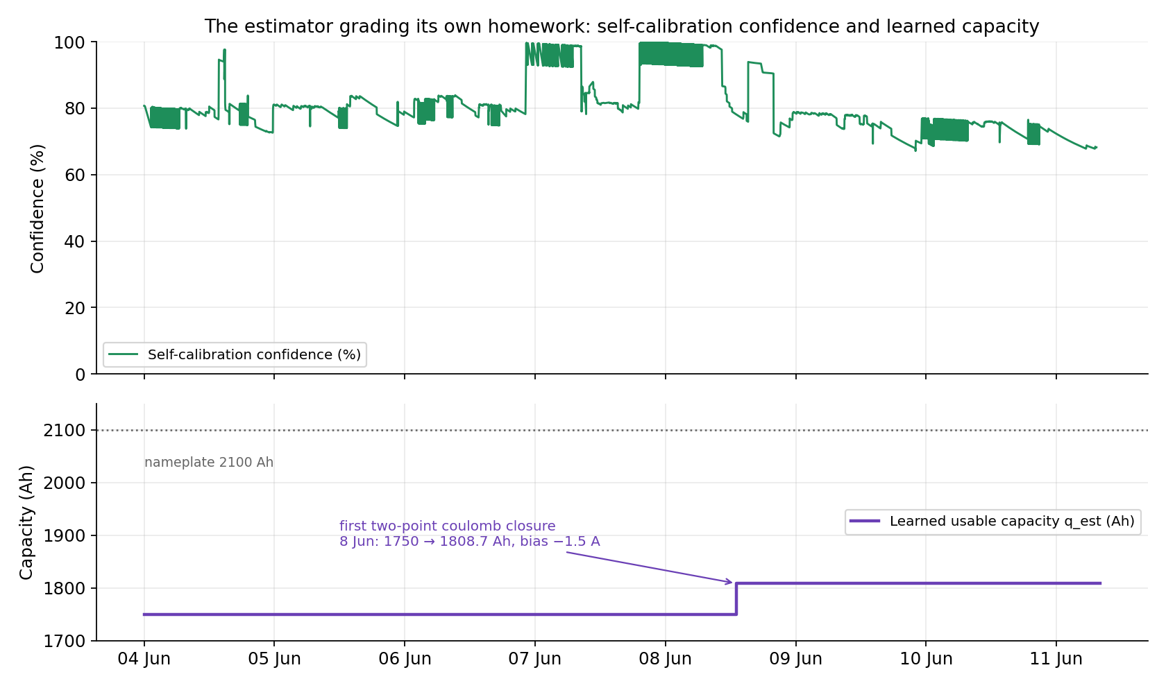
The estimator grading its own homework. Top: a week of the published confidence score — rising on fresh anchors, decaying as they age. Bottom: the learned usable capacity, with the first two-point coulomb closure on 8 June stepping it from 1750 to 1808.7 Ah — measured, not assumed, against a 2100 Ah nameplate.

The same layer guards itself. Closures are rejected unless the anchors were genuinely rested (a closure attempted under 38 A of load gets thrown away). New capacity observations move the estimate slowly — one noisy closure can’t yank it. And when the pack rests near the discharge floor, a deep-low capture fires autonomously — the box runs 24/7, so the calibration improves without anyone touching anything.

One mistake from this period is worth confessing publicly because the failure mode is general: we once injected a historical rest point into the live closure path, and the layer dutifully closed the loop between a real anchor and a fake one — instantly corrupting the learned capacity by 180 Ah. It was caught and reverted within minutes, but the lesson stands: never feed live calibration machinery a data point from the past. Historical points now go through a separate path that can only adjust the OCV table, never the live capacity.

Mining 21 months of history for free anchors

The recorder on the Home Assistant box turned out to hold hourly battery statistics back to September 2024 — 21 months of voltage and current. Mining it produced the kind of calibration data you normally need a lab for:

• 77 deep-discharge events, and at every single one the BMS cutoff sat at 2.80 V/cell (44.8 V pack) at near-zero current — rock-stable across 21 months and all seasons. The hardware floor is a fixed voltage threshold, and there is no detectable low-end degradation.
• 69 full-charge absorption events at 3.45–3.51 V/cell, and a relaxed-empty OCV of ~2.95 V/cell — both now seeded into the learned OCV table through the historical-ingest path.

That 2.80 V floor line appears in the next chart, doing real work.

Falsifying the whole stack on purpose: the off-grid deep discharge

After the oscillation night there was no honest way to re-anchor the inverter’s counter except to take the pack to a reference point the Deye itself recognises. So we made one: physically isolate the grid and let the house run the battery down toward the BMS floor — a deliberate, supervised version of the event the whole project exists to prevent.

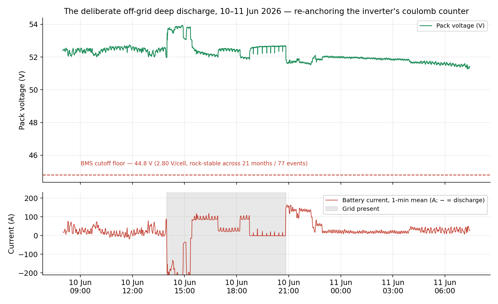
The deliberate off-grid discharge, 10–11 June. Top: pack voltage grinding down, with the BMS floor at 44.8 V — the line 77 historical events say is exact — still far below. Bottom: battery current, with discharge pushes past 150 A (~8 kW) while the house runs entirely on the pack; the shaded band is a brief grid-restore window. Throughout this, the inverter’s SOC read 0 % and the estimator carried the house on its own number.

This exercise is also a stress test the estimator passed in a way no dashboard demo could. For the whole period the Deye reported 0 % — the pack meanwhile delivering 8 kW for hours. The estimator tracked smoothly down through 50 %, 40 %, 25 %, on nothing but its learned capacity, learned bias and gated coulomb counting. LFP being LFP, the pack voltage spent almost the entire discharge between 54 and 51 V — the plateau problem again, live: voltage alone cannot tell 55 % from 25 %. Only a calibrated counter can. At the time of writing the pack is still grinding toward the floor; when it gets there, the inverter’s counter re-anchors at a true zero and the estimator’s deep-low capture takes a fresh anchor automatically.

The cut-over — and what guards it

On 10 June the optimiser’s starting-SOC input was re-pointed from the inverter’s register to sensor.dekf_soc, and its energy model updated to the measured 92.6 kWh. That is the whole integration: one config line, because the estimator was built as a first-class HA sensor from day one. The second opinion is now the planning number.

What guards it is more interesting than the cut-over itself:

• The hardware BMS floor is untouched and unconditional — the 2.80 V/cell cutoff that 77 historical events show firing at exactly the same voltage. Software never relaxes a hardware limit.
• The inverter SOC stays alive as a permanent cross-check. Divergence beyond a threshold flags a fault and falls back to the more conservative reading — the quarantine guard from the original design, now with one crucial refinement: the fallback first sanity-checks the inverter’s number and refuses to inherit a pinned 0 % or clamped 100 %. A conservative min(a, b) rule is worse than useless when one input is garbage at zero.
• Register writes got an arbiter. A post-incident audit found six independent pieces of software — the optimiser’s automation, the charge controller, mode scripts, the calibration campaign — all writing to the same handful of inverter registers with no coordination. Nearly every control bug in the project’s history, the oscillation night included, was two writers disagreeing. A single arbiter now sits in front of the registers with strict priorities and hard interlocks, the most important being: never zero the discharge current while the grid is absent — off-grid, that command is a self-inflicted house blackout. It runs in shadow mode first, logging what it would have done; within 90 seconds of deployment it correctly refused exactly that blackout-inducing write while the house was islanded.
• Blackout-safe restarts. Because the battery is the house UPS here, the estimator must reboot sanely after a blackout. On restart it seeds from rested OCV if it can, falls back to the inverter only after sanity checks, and widens its own uncertainty so the first anchors pull it in fast.

The external reviewer’s verdict on the revised architecture, for what an argumentative critic’s endorsement is worth: no critical safety or correctness flaws in the core concept, and a system “better than most home LFP + Deye/HA setups” it had seen documented.

Why a Pi/HA box is the right place for this

Three reasons it isn’t a hardware project.

The compute requirement is trivial. The filter is three floats of state and a 3×3 covariance; one step takes microseconds. The Home Assistant Green box (ARM64, 4 GB RAM) sits at ~5 % CPU even with EMHASS, the Sunsynk integration, the energy dashboard, the estimator, the self-calibration layer and a dozen automations running. The entire estimation stack is a few Python files. For non-Pi readers running Home Assistant on a NUC, Mac mini or home server box, the same applies.

The integration is data, not wires. The stack reads pack voltage and current from sensors that already exist in HA (sensor.sunsynk2_battery_voltage, sensor.battery_current_total_inv2_inv3), runs the filter, and publishes new sensors. Nothing physical changes; nothing about the inverter’s wiring or the battery’s BMS is altered.

And the data you already have is an asset. The 21-month recorder archive gave us the BMS floor characterisation and OCV seed points for free — data that was sitting in a SQLite file the whole time.

Why this matters for everyone running a home battery

The same pattern applies to anyone running an LFP battery against a real-time tariff. The chemistry is the same. The OCV plateau is the same. The drift problem is the same — and as our week of 0 %-and-100 % shows, it is not a gentle few-percent error; a coulomb counter anchored from a bad reference is wrong by fifty points with total confidence. The hardware BMS limits are your only safety floor, and you only want them to fire in genuine emergencies, not because the software optimisation layer is working from a fictional number. Time-of-use tariff arbitrage makes accurate SOC matter more, not less: aggressive cycling assumes the cycles are landing where you think they are, and the oscillation night shows what “where you think they are” costs — a night of grid import with 45 kWh sitting idle.

If you are building a BESS yourself from prismatic LFP cells, or sourcing the printed-circuit-board assemblies for monitoring hardware, the calibration story above is the gap between “this works as well as the spec sheet says” and “this works as well as a major manufacturer’s product”. For commercial-scale installs that ship globally, the same component-sourcing discipline applies at every level of the stack. For Australian installs in particular, local supply chains for the inverter and battery side make iteration cycles much faster.

What’s next

The stack is live but young. The confidence score still decays between anchors; the next clean floor rest fires an autonomous capture and, with it, a second capacity closure on a cleaner swing than the first. The arbiter graduates from shadow to enforcement one writer at a time. On the filter-physics side the backlog is real but unhurried: a second RC branch for slow diffusion polarisation, capacity fade tracking from charge-curve analysis, and a string-imbalance check for the 21 parallel modules. The story arc — the over-discharge near-miss, the drift diagnosis, the filter build, the external review, the self-calibration pivot, the oscillation night, the cut-over — continues here as it happens.

Get the code

The full production stack is open-sourced under MIT: github.com/borntobefree2-cmyk/dekf-lfp-soc — the estimator, the self-calibration layer, the OCV campaign manager and the register arbiter, byte-identical to the deployment described above (md5s in the README), plus an install walk-through and the safety notes you should read first. If your inverter exposes pack voltage and current to Home Assistant, you can run the same second opinion this post is about.

FAQ

Why not just use a closed-loop CAN BMS? It is the correct long-term architecture and we will probably end up there. The Deye accepts Pylontech-format CAN telemetry; an ESP32-based aggregator that filters single-module alarms and presents one clean frame is well-trodden ground. It is a 1–2 week hardware project, though. The software estimator got most of the win in software, on a box we already own — and the self-calibration layer means it keeps getting better without further effort.

Why a Kalman filter and not machine learning? Filter-based and ML approaches both exist; some are excellent. The closest structural match to the failure mode this post describes is the Fisher-information fusion approach from Shi, Moura and colleagues (2025), which weighs coulomb counting and ECM identification by current-excitation informativeness — directly attacking the current-bias-dominated drift we observe. We chose a Plett-style EKF because it is interpretable, debuggable from first principles, and small enough to fit on the same box that runs everything else. Every parameter has a physical meaning — which is precisely what made the stale-parameter diagnosis, and therefore the self-calibration pivot, possible. A black box cannot tell you which of its constants is lying.

What’s the actual accuracy? Near full it tracks within a fraction of a percent. Through the mid-band it is governed by the learned capacity and bias — and the first closure measured those to 1808.7 Ah and −1.5 A respectively, with a confidence score published alongside so you always know how fresh the calibration is. The honest residual: capacity is a young estimate (one closure, deliberately slow-moving); expect it to refine over the next few clean cycles. The old below-30 % failure mode traced to stale parameters and steep-zone anchoring discipline, both now addressed; the deliberate deep discharge above is what its replacement looks like under stress.

Isn’t the DEKF a single point of failure once EMHASS depends on it? No, by design. The inverter SOC stays alive as a permanent cross-check with a conservative fallback (sanity-checked, so a pinned 0 % can’t poison it), a register arbiter enforces safe writes with an islanding interlock, and the hardware BMS limits sit below all of it as the actual safety floor. The estimator is an additional SOC source that earned the planning role — not an unguarded replacement.

Can I run this on my system? If your inverter exposes battery voltage and current to Home Assistant as sensors (most Sunsynk / Deye / Solis / Victron addons do), yes. The estimator and its self-calibration layer are AppDaemon apps. You no longer need to hand-fit capacity and the OCV curve — teaching itself those numbers from your pack’s ordinary operation is exactly what the calibration layer is for. You do need patience: the first capacity closure needs the pack to visit both a rested low point and a rested high point.

How much did it cost? Zero new hardware. The original filter was about ten hours of Python; the self-calibration layer and arbiter roughly doubled that. A Home Assistant Green is ~AUD 200 if you do not already have one — but if you are running EMHASS and a battery you almost certainly do.

Glossary

• BMS — Battery Management System. The electronics that monitor cells and enforce hard safety limits.
• SOC — State of Charge. The percentage of usable energy left in the pack.
• OCV — Open-Circuit Voltage. The terminal voltage when no current is flowing — the cleanest signal you have on a battery’s true state.
• ECM — Equivalent-Circuit Model. The standard lumped-parameter battery model: a voltage source (OCV), a series resistance (R0) and one or more RC pairs (polarisation).
• EKF / DEKF — Extended Kalman Filter / Dual Extended Kalman Filter. A recursive state estimator for non-linear systems; the “Dual” variant tracks parameter drift alongside state.
• EMHASS — Energy Management Home Assistant System. The open-source Model-Predictive-Control optimiser that schedules the battery against forecasts and prices.
• LFP / LiFePO₄ — Lithium iron phosphate. Long-cycle-life lithium chemistry with the flat-OCV plateau that makes SOC estimation hard.
• Plett-style — A family of battery-state estimators described in Gregory Plett’s 2004 Journal of Power Sources papers, the foundational reference for EKF-based battery management.
• Two-point coulomb closure — Capacity measurement from two rested anchors: the Amp-hours integrated between a known low SOC and a known high SOC yield true capacity and current bias jointly.
• Quarantine guard — A permanent comparison process that keeps the inverter SOC alive as a cross-check after the DEKF takes over EMHASS’s soc_init. Falls back to the more conservative sane reading when they disagree.
• Register arbiter — A single gatekeeper through which all software writes to the inverter’s control registers pass, enforcing priorities, rate limits and safety interlocks (chief among them: never zero discharge while off-grid).

This is part of an ongoing series on home battery optimisation. Previous posts: Energy Arbitrage Explained, Amber Electric — Review, Amber Electric Australia + Home Battery.